Sep 2, 2015 | excel, Excel functions, Excel tips, if condition, if formula, ms excel, multiple conditions, office excel
Excel IF function with multiple conditions
this article had taken from this source
In Part 1 of our Excel IF function tutorial, we started to learn the nuts and bolts of the Excel IF function. As you remember, we discussed a few IF formulas for numbers, dates and text values as well as how to use the IF function with blank and non-blank cells.
However, for powerful data analysis, you may often need to evaluate multiple conditions at a time, meaning you have to construct more sophisticated logical tests using multiple IF functions in one formula. The formula examples that follow below will show you how to do this correctly. You will also learn how to use Excel IF in array formulas and learn the basics of the IFEFFOR and IFNA functions.
How to use Excel IF function with multiple conditions
In summary, there can be 2 basic types of multiple conditions – with AND and OR logic. Consequently, your IF function should embed an AND or OR function in the logical test, respectively.
- AND function. If your logical test contains the AND function, Microsoft Excel returns TRUE if all the conditions are met; otherwise it returns FALSE.
- OR function. In case you use the OR function in the logical test, Excel returns TRUE if any of the conditions is met; FALSE otherwise.
To illustrate the point better, let’s have a look at a few IF examples with multiple conditions.
Example 1. Using IF & AND function in Excel
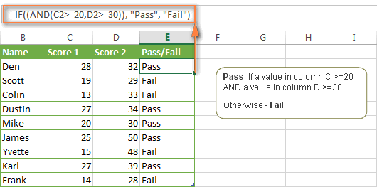
Suppose, you have a table with the results of two exam scores. The first score, stored in column C, must be equal to or greater than 20. The second score, listed in column D, must be equal to or exceed 30. Only when both of the above conditions are met, a student passes the final exam.
The easiest way to make a proper formula is to write down the condition first, and then incorporate it in the logical_test argument of your IF function:
Condition: AND(B2>=20, C2>=30)
IF/AND formula: =IF((AND(C2>=20, D2>=30)), "Pass", "Fail")
Easy, isn’t it? The formula tells Excel to return “Pass” if a value in column C >=20 AND a value in column D >=30. Otherwise, the formula returns “Fail”. The screenshot below proves that our Excel IF /AND function is correct:
Note. Microsoft Excel checks all conditions in the AND function, even if one of the already tested conditions evaluates to FALSE. Such behavior is a bit unusual since in most of programming languages, subsequent conditions are not tested if any of the previous tests has returned FALSE.
In practice, a seemingly correct IF / AND formula may result in an error because of this specificity. For example, the formula =IF(AND(A2<>0,(1/A2)>0.5),”Good”, “Bad”) will return “Divide by Zero Error” (#DIV/0!) if cell A2 is equal to 0. The avoid this, you should use a nested IF function: =IF(A2<>0, IF((1/A2)>0.5, “Good”, “Bad”), “Bad”)
Example 2. Using IF with OR function in Excel
You use the combination of IF & OR functions in a similar way. The difference from the IF / AND formula discussed above is that Excel returns TRUE if at least one of the specified conditions is met.
So, if we modify the above formula in the following way:
=IF((OR(C2>=20, D2>=30)), "Pass", "Fail")
Column E will have the “Pass” mark if either the first score is equal to or greater than 20 OR the second score is equal to or greater than 30.
As you see in the screenshot below, our students have a better chance to pass the final exam with such conditions (Scott being particularly unlucky failing by just 1 point : )

Naturally, you are not limited to using only two AND/OR functions in your Excel IF formulas. You can use as many logical functions as your business logic requires, provided that:
- In Excel 2013, 2010 and 2007, your formula includes no more than 255 arguments, and the total length of the formula does not exceed 8,192 characters.
- In Excel 2003 and lower, you can use up to 30 arguments and the total length of your formula shall not exceed 1,024 characters.
Example 3. Using IF with AND & OR functions
In case you have to evaluate your data based on several sets of multiple conditions, you will have to employ both AND & OR functions at a time.
In the above table, suppose you have the following criteria to evaluate the students’ success:
- Condition 1: column C>=20 and column D>=25
- Condition 2: column C>=15 and column D>=20
If either of the above conditions is met, the final exam is deemed passed, otherwise – failed.
The formula might seem tricky, but in a moment, you will see that it is not! You just have to express two conditions as AND statements and enclose them in the OR function since you do not require both conditions to be met, either will suffice:
OR(AND(C2>=20, D2>=25), AND(C2>=15, D2>=20)
Finally, use the above OR function as the logical test in the IF function and supply value_if_true and value_if_false arguments. As the result, you will get the following IF formula with multiple AND / OR conditions:
=IF(OR(AND(C2>=20, D2>=25), AND(C2>=15, D2>=20)), "Pass", "Fail")
The screenshot below indicates that we’ve got the formula right:

Using multiple IF functions in Excel (nested IF functions)
If you need to create more elaborate logical tests for your data, you can include additional IF statements in the value_if_true and value_if_false arguments of your Excel IF formulas. These multiple IF functions are called “nested IF functions” and they may prove particularly useful if you want your formula to return 3 or more different results.
Here’s an easy-to-understand example. Suppose you want not simply to qualify the students’ results as Pass/Fail, but rather define the total score as “Good“, “Satisfactory” and “Poor“. For example:
- Good: 60 or more (>=60)
- Satisfactory: between 40 and 60 (>40 and <60)
- Poor: 40 or less (<=40)
To begin with, you can add an additional column (E) with the following formula that sums numbers in columns C and D: =C2+D2

And now, let’s write a nested IF function based on the above conditions. It’s considered a good practice to start with the most important condition and make your functions as simple as possible. Our Excel nested IF formula is as follows:
=IF(E2>=60, "Good", IF(E2>40, "Satisfactory", "Poor "))
As you see, just one nested IF function is sufficient in this case. Naturally, you can nest more IF functions if you want to. For example:
=IF(E2>=70, "Excellent", IF(E2>=60, "Good", IF(E2>40, "Satisfactory", "Poor ")))
The above formula adds one more conditions – the total score of 70 points and more is qualified as “Excellent”.

I’ve heard some people say that multiple Excel IF functions are driving them crazy : ) Probably, it will help if you try to look at our nested IF formula in this way:

What the formula actually tells Excel to do is to test the condition of the first IF function and return the value supplied in the value_if_true argument if the condition is met. If the condition of the 1st IF function is not met, then test the 2nd IF, and so on.
=IF(check if E2>=70, if true – return “Excellent”, or else
IF(check if E2>=60, if true – return “Good”, or else
IF(check if E2>40, if true – return “Satisfactory”, if false
– return ” Poor “)))
Excel nested IF functions – things to remember!
1. In modern versions of Excel 2013, 2010 and 2010, you can use up to 64 nested IF functions. In older versions of Excel 2003 and lower, up to 7 nested IF functions can be used.
2. If your IF formula includes more than 5 nested IF functions, you may want to optimize it by using the alternatives described below.
Alternatives to multiple IF functions in Excel
To get around the limit of seven nested IF functions in older Excel versions and to make your IF formula more compact and fast, consider using the following approaches instead of multiple IF statements.
1. To test many conditions, use the LOOKUP, VLOOKUP, INDEX/MATCH or CHOOSE functions.
2. Use IF with logical functions OR / AND, as demonstrated in the above examples.
3. Use the CONCATENATE function or the concatenate operator (&).
As well as other Excel functions, CONCATENATE can include as many as 30 parameters in older Excel versions and up to 255 arguments in modern versions, which equates to testing 255 different conditions.
For example, if you want to return different values depending on the content of cell B1, you can use the following formulas:
Nested IF functions:
=IF(C1="a", "Excellent", IF(C1="b", "Good", IF(C1="c", "Poor", "")))
CONCATENATE function:
=CONCATENATE(IF(C1="a", "Excellent", ""), IF(C1="b", "Good", ""), IF(C1="c", "Poor ", ""))
Concatenate operator:
=IF(C1="A", "Excellent", "") & IF(C1="B", " Good", "") & IF(C1="C", "Poor", "")
As you see, the use of CONCATENATE does not make the formula shorter, but it does make it easier-to-understand compared to nested IF functions.

4. For powerful Excel users, the best alternative to using multiple nested IF functions might be creating a custom worksheet function using VBA.
Using Excel IF in array formulas
Like other Excel functions, IF can be used in array formulas. You may need such a formula if you want to evaluate every element of the array when the IF statement is carried out.
For example, the following array SUM/IF formula demonstrates how you can sum cells in the specified range based on a certain condition rather than add up the actual values:
=SUM(IF(B1:B5<=1,1,2))
The formula assigns a certain number of “points” to each value in column B – if a value is equal to or less than 1, it equates to 1 point; and 2 points are assigned to each value greater than 1. And then, the SUM function adds up the resulting 1’s and 2’s, as shown in the screenshot below.

Note. Since this is an array formula, remember to press Ctrl + Shift + Enter to enter it correctly.
Using IF function together with other Excel functions
Earlier in this tutorial, we’ve discussed a few IF formula examples demonstrating how to use the Excel IF function with logical functions AND and OR. Now, let’s see what other Excel functions can be used with IF and what benefits this gives to you.
Example 1. Using IF with SUM, AVERAGE, MIN and MAX functions
When discussing nested IF functions, we wrote the formula that returns different ranking (Excellent, Good, Satisfactory or Poor) based on the total score of each student. As you remember, we added a new column with the formula that calculates the total of scores in columns C and D.
But what if your table has a predefined structure that does not allow any modifications? In this case, instead of adding a helper column, you could add values directly in your If formula, like this:
=IF((C2+D2)>=60, "Good", IF((C2+D2)>=>40, "Satisfactory", "Poor "))
Okay, but what if your table contains a lot of individual scores, say 5 different columns or more? Summing so many figures directly in the IF formula would make it enormously big. An alternative is embedding the SUM function in the IF’s logical test, like this:
=IF(SUM(C2:F2)>=120, "Good", IF(SUM(C2:F2)>=90, "Satisfactory", "Poor "))

In a similar fashion, you can use other Excel functions in the logical test of your IF formulas:
IF and AVERAGE:
=IF(AVERAGE(C2:F2)>=30,"Good",IF(AVERAGE(C2:F2)>=25,"Satisfactory","Poor "))
The formulas retunes “Good” if the average score in columns C:F is equal to or greater than 30, “Satisfactory” if the average score is between 29 and 25 inclusive, and “Poor” if less than 25.
IF and MAX/MIN:
To find the highest and lowest scores, you can use the MAX and MIN functions, respectively. Assuming that column F is the total score column, the below formulas work a treat:
MAX: =IF(F2=MAX($F$2:$F$10), "Best result", "")
MIN: =IF(F2=MIN($F$2:$F$10), "Worst result", "")
If you’d rather have both the Min and Max results in the same column, you can nest one of the above functions in the other, for example:
=IF(F2=MAX($F$2:$F$10) ,"Best result", IF(F2=MIN($F$2:$F$10), "Worst result", ""))

In a similar manner, you can use the IF function with your custom worksheet functions. For example, you can use it with the GetCellColor / GetCellFontColor functions to return different results based on a cell color.
In addition, Excel provides a number of special IF functions to analyze and calculate data based on different conditions.
For example, to count the occurrences of a text or numeric value based on a single or multiple conditions, you can use COUNTIF and COUNTIFS, respectively. To find out a sum of values based on the specified condition(s), use the SUMIF or SUMIFS functions. To calculate the average according to certain criteria, use AVERAGEIF or AVERAGEIFS.
For the detailed step-by-step formula examples, check out the following tutorials:
Example 2. IF with ISNUMBER and ISTEXT functions
You already know a way to spot blank and non-blank cells using the ISBLANK function. Microsoft Excel provides analogous functions to identify text and numeric values – ISTEXT and ISNUMBER, respectively.
Here’s is example of the nested Excel IF function that returns “Text” if cell B1 contains any text value, “Number” if B1 contains a numeric value, and “Blank” if B1 is empty.
=IF(ISTEXT(B1), "Text", IF(ISNUMBER(B1), "Number", IF(ISBLANK(B1), "Blank", "")))

Note. Please pay attention that the above formula displays “Number” for numeric values and dates. This is because Microsoft Excel stores dates as numbers, starting from January 1, 1900, which equates to 1.
Example 3. Using the result returned by IF in another Excel function
Sometimes, you can achieve the desired result by embedding the IF statement in some other Excel function, rather than using another function in a logical test.
Here’s another way how you can use the CONCATINATE and IF functions together:
=CONCATENATE("You performed ", IF(C1>5,"fantastic!", "good"))
I believe you hardly need any explanation of what the formula does, especially looking at the screenshot below:

Excel IFERROR and IFNA functions
Both of the functions – IFERROR and IFNA – are used in Excel to trap errors in formulas. And both functions can return a special value that you specify if a formula produces an error. Otherwise, the result of the formula is returned.
The difference is that IFERROR handles all possible Excel errors, including #VALUE!, #N/A, #NAME?, #REF!, #NUM!, #DIV/0!, and #NULL!. While the Excel IFNA function specializes solely in #N/A errors, exactly as its name suggests.
The syntax of the Error functions is as follows.
IFERROR function
IFERROR(value, value_if_error)
IFNA function
IFNA(value, value_if_na)
The first parameter (value) is the argument that is checked for an error.
The second parameter (value_if_error / value_if_na) is the value to return if the formula evaluates to an error (any error in case of IFERROR; the #N/A error in case of IFNA).
Note. If any of the arguments is an empty cell, both of the Error functions treat it as an empty string (“”).
The following example demonstrates the simplest usage of the IFERROR function:
=IFERROR(B2/C2, "Sorry, an error has occurred")

As you see in the screenshot above, column D displays the quotient of the division of a value in column B by a value in column C. You can also see two error messages in cells D2 and D5 because everyone knows that you cannot divide a number by zero.
In some cases, you’d better use the IF function to prevent an error then ISERROR or ISNA to catch an error. Firstly, it’s a faster way (in terms of CPU) and secondly it is a good programming practice. For example, the following IF formula produces the same result as the IFERROR function demonstrated above:
=IF(C2=0, "Sorry, an error has occurred", B2/C2)
But of course, there are cases when you cannot pre-test all function parameters, especially in very complex formulas, and foresee all possible errors. In such cases, the ISERROR() and IFNA() functions come in really handy. You can find a few advanced examples of using IFERROR in Excel in these articles:
And that’s all I have to say about using the IF function in Excel. Hopefully, the IF examples we’ve discussed in this tutorial will help you to get started on the right track. Thank you for reading!