Feb 11, 2016 | area, ccna, exam, Learn and Teach, OSPF, OSPF Questions 2, question, Quiz, test
CCNP ROUTE Practice Exam:
Multiarea OSPF 4
Chris Bryant, “The Computer Certification Bulldog”
Here’s the 4th practice exam in this series. Dig in!
Question 1:
You’re configuring an OSPF ASBR, and have determined that all the routes injected into OSPF via redistribution can be summarized with the address 23.0.0.0 /12.
What is the full OSPF command to advertise this summary into the OSPF domain in place of the specific routes?
Question 2:
You’re performing two-way route redistribution between an EIGRP AS and an OSPF domain. On the OSPF routers, what is the default routing table code for the routes learned from EIGRP?
Extra credit: What code will appear on the EIGRP routers next to any routes that are injected into the EIGRP AS from OSPF?
Consider the following OSPF configuration and answer the following questions.
R4(config)#router ospf 1
R4(config-router)#network 172.12.0.0 0.0.0.255 area 0
R4(config-router)#network 1.1.1.1 0.0.0.0 area 1
R4(config-router)#router-id 20.1.1.1
< router reloaded at this point >
R4(config)#interface loopback0
R4(config-if)#ip address 50.1.1.1 255.255.255.255
Question 3:
Is that a legal configuration? If not, why not?
Question 4:
What is the OSPF process number?
Question 5:
What is the RID of this particular router?
Question 6:
Is this router an ABR, ASBR, both, or neither?
Explain why this router is or isn’t an ABR.
Explain why this router is or isn’t an ASBR.
This ends the questions about that router configuration.
Question 7:
An OSPF total stub router can contain what route types?
A. Default route only
B. E2 routes and a default route
C. E1 routes and a default route
D. Intra-area routes and a default route
E. Inter-area routes and a default route
Answers:
1. The full command is:
summary-address 23.0.0.0 255.240.0.0
2. These routes will appear as OSPF External Type 2 routes and will have a router table code of “O E2”.
The routes that are redistributed from OSPF into EIGRP will appear in the EIGRP routing tables with a code of “D EX”.
3. Yep, it’s legal.
4. The OSPF process number is 1, as indicated by the router ospf 1 command.
5. The OSPF RID was hardcoded as 20.1.1.1, and it took effect after the router reload I mentioned.
6. This router is an ABR since it borders Area 1 and Area 0.
There is no route redistribution shown on this router, so it’s not an ASBR.
7. “D”. The routing table of a total stub router can contain intra-area routes and a default inter-area route using the ABR as the next hop.
Thanks for taking this CCNP practice exam – here are the other OSPF multiarea exams!
Feb 11, 2016 | ccna, exam, Learn and Teach, Networking, OSPF, OSPF Questions 2, questions, Quiz, test
Question 1
Into which two types of areas would an area border router (ABR) inject a default route? (Choose two)
A. the autonomous system of a different interior gateway protocol (IGP)
B. area 0
C. totally stubby
D. NSSA
E. stub
F. the autonomous system of an exterior gateway protocol (EGP)
Answer: C E
Explanation
Both stub area & totally stubby area allow an ABR to inject a default route. The main difference between these 2 types of areas is:
+ Stub area replaces LSA Type 5 (External LSA – created by an ASBR to advertise network from another autonomous system) with a default route
+ Totally stubby area replaces both LSA Type 5 and LSA Type 3 (Summary LSA – created by an ABR to advertise network from other areas, but still within the AS, sometimes called interarea routes) with a default route.
Below summarizes the LSA Types allowed and not allowed in area types:
| Area Type |
Type 1 & 2 (within area) |
Type 3 (from other areas) |
Type 4 |
Type 5 |
Type 7 |
| Standard & backbone |
Yes |
Yes |
Yes |
Yes |
No |
| Stub |
Yes |
Yes |
No |
No |
No |
| Totally stubby |
Yes |
No |
No |
No |
No |
| NSSA |
Yes |
Yes |
No |
No |
Yes |
| Totally stubby NSSA |
Yes |
No |
No |
No |
Yes |
Question 2
Which three restrictions apply to OSPF stub areas? (Choose three)
A. No virtual links are allowed.
B. The area cannot be a backbone area.
C. Redistribution is not allowed unless the packet is changed to a type 7 packet.
D. The area has no more than 10 routers.
E. No autonomous system border routers are allowed.
F. Interarea routes are suppressed.
Answer: A B E
Question 3
Refer to the partial configurations in the exhibit. What address is utilized for DR and BDR identification on Router1?
| Router1#show run**** output omitted ******
interface serial1/1
ipv6 address 2001:410:FFFE:1::64/64
ipv6 ospf 100 area 0
!
interface serial2/0
ipv6 address 3FFF:B00:FFFF:1::2/64
ipv6 ospf 100 area 0
!
ipv6 router ospf
router-id 10.1.1.3 |
A. the serial 1/1 address
B. the serial 2/0 address
C. a randomly generated internal address
D. the configured router-id address
Answer: D
Explanation
In OSPFv3 and OSPF version 2, the router uses the 32-bit IPv4 address to select the router ID for an OSPF process. The router ID selection process for OSPFv3 is described below (same as OSPF version 2):
1. The router ID is used if explicitly configured with the router-id command.
2. Otherwise, the highest IPv4 loopback address is used.
3. Otherwise, the highest active IPv4 address.
4. Otherwise, the router ID must be explicitly configured.
In this case the router ID 10.1.1.3 is explicitly configured -> D is correct.
Question 4
By default, which statement is correct regarding the redistribution of routes from other routing protocols into OSPF?
A. They will appear in the OSPF routing table as type E1 routes.
B. They will appear in the OSPF routing table as type E2 routes.
C. Summarized routes are not accepted.
D. All imported routes will be automatically summarized when possible.
E. Only routes with lower administrative distances will be imported.
Answer: B
Explanation
Type E1 external routes calculate the cost by adding the external cost to the internal cost of each link that the packet crosses while the external cost of E2 packet routes is always the external cost only. E2 is useful if you do not want internal routing to determine the path. E1 is useful when internal routing should be included in path selection. E2 is the default external metric when redistributing routes from other routing protocols into OSPF -> B is correct.
Question 5
Which statement is true about OSPF Network LSAs?
A. They are originated by every router in the OSPF network. They include all routers on the link, interfaces, the cost of the link, and any known neighbor on the link.
B. They are originated by the DR on every multi-access network. They include all attached routers including the DR itself.
C. They are originated by Area Border Routers and are sent into a single area to advertise destinations outside that area.
D. They are originated by Area Border Router and are sent into a single area to advertise an Autonomous System Border Router.
Answer: B
Explanation
Popular LSA Types are listed below:
| LSA Type |
Description |
Details |
| 1 |
Router LSA |
Generated by all routers in an area to describe their directly attached links |
| 2 |
Network LSA |
Advertised by the DR of the broadcast network (does not cross ABR) |
| 3 |
Summary LSA |
Advertised by the ABR of originating area |
| 4 |
Summary LSA |
Generated by the ABR of the originating area to advertise an ASBR to all other areas in the autonomous system |
| 5 |
AS external LSA |
Used by the ASBR to advertise networks from other autonomous systems |
| 7 |
Defined for NSSAs |
Generated by an ASBR inside a Not-so-stubby area (NSSA) to describe routes redistributed into the NSSA |
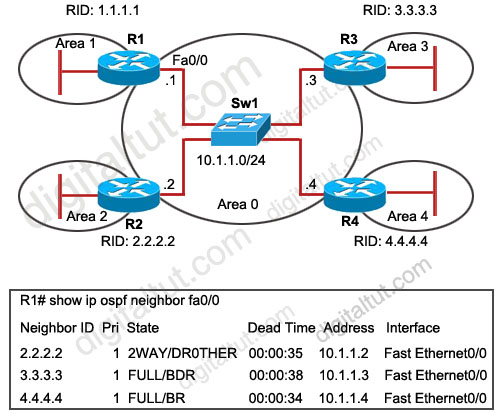
Question 6
Refer to the exhibit. OSPF is configured on all routers in the network. On the basis of the show ip ospf neighbor output, what prevents R1 from establishing a full adjacency with R2?

A. Router R1 will only establish full adjacency with the DR and BDR on broadcast multiaccess networks.
B. Router R2 has been elected as a DR for the broadcast multiaccess network in OSPF area
C. Routers R1 and R2 are configured as stub routers for OSPF area 1 and OSPF area 2.
D. Router R1 and R2 are configured for a virtual link between OSPF area 1 and OSPF area 2.
E. The Hello parameters on routers R1 and R2 do not match.
Answer: A
Explanation
From the output, we learn that R4 is the DR and R3 is the BDR so other routers will only establish full adjacency with these routers. All other routers have the two-way adjacency established -> A is correct.
Question 7
Refer to the exhibit. On the basis of the configuration provided, how are the Hello packets sent by R2 handled by R5 in OSPF area 5?
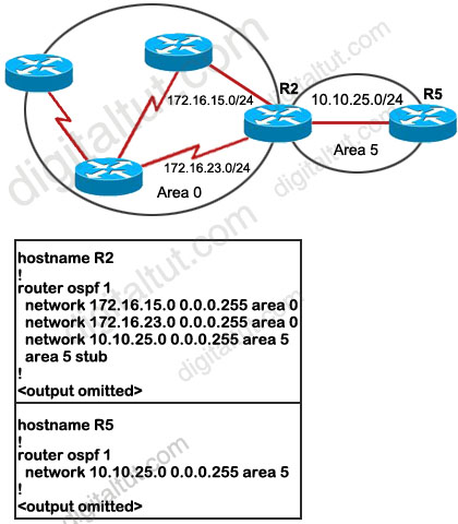
A. The Hello packets will be exchanged and adjacency will be established between routers R2 and R5.
B. The Hello packets will be exchanged but the routers R2 and R5 will become neighbors only.
C. The Hello packets will be dropped and no adjacency will be established between routers R2 and R5.
D. The Hello packets will be dropped but the routers R2 and R5 will become neighbors.
Answer: C
Explanation
Recall that in OSPF, two routers will become neighbors when they agree on the following: Area-id, Authentication, Hello and Dead Intervals, Stub area flag.
We must specify Area 5 as a stub area on the ABR (R2) and all the routers in that area (R5 in this case). But from the output, we learn that only R2 has been configured as a stub for Area 5. This will drop down the neighbor relationship between R2 and R5 because the stub flag is not matched in the Hello packets of these routers.
Question 8
When an OSPF design is planned, which implementation can help a router not have memory resource issues?
A. Have a backbone area (area 0) with 40 routers and use default routes to reach external destinations.
B. Have a backbone area (area 0) with 4 routers and 30,000 external routes injected into OSPF.
C. Have less OSPF areas to reduce the need for interarea route summarizations.
D. Have multiple OSPF processes on each OSPF router. Example, router ospf 1, router ospf 2
Answer: A
Question 9
When verifying the OSPF link state database, which type of LSAs should you expect to see within the different OSPF area types? (Choose three)
A. All OSPF routers in stubby areas can have type 3 LSAs in their database.
B. All OSPF routers in stubby areas can have type 7 LSAs in their database.
C. All OSPF routers in totally stubby areas can have type 3 LSAs in their database.
D. All OSPF routers in totally stubby areas can have type 7 LSAs in their database.
E. All OSPF routers in NSSA areas can have type 3 LSAs in their database.
F. All OSPF routers in NSSA areas can have type 7 LSAs in their database.
Answer: A E F
Explanation
Below summarizes the LSA Types allowed and not allowed in area types:
| Area Type |
Type 1 & 2 (within area) |
Type 3 (from other areas) |
Type 4 |
Type 5 |
Type 7 |
| Standard & backbone |
Yes |
Yes |
Yes |
Yes |
No |
| Stub |
Yes |
Yes |
No |
No |
No |
| Totally stubby |
Yes |
No |
No |
No |
No |
| NSSA |
Yes |
Yes |
No |
No |
Yes |
| Totally stubby NSSA |
Yes |
No |
No |
No |
Yes |
Popular LSA Types are listed below:
| LSA Type |
Description |
Details |
| 1 |
Router LSA |
Generated by all routers in an area to describe their directly attached links |
| 2 |
Network LSA |
Advertised by the DR of the broadcast network (does not cross ABR) |
| 3 |
Summary LSA |
Advertised by the ABR of originating area |
| 4 |
Summary LSA |
Generated by the ABR of the originating area to advertise an ASBR to all other areas in the autonomous system |
| 5 |
AS external LSA |
Used by the ASBR to advertise networks from other autonomous systems |
| 7 |
Defined for NSSAs |
Generated by an ASBR inside a Not-so-stubby area (NSSA) to describe routes redistributed into the NSSA |
Question 10
You are troubleshooting an OSPF problem where external routes are not showing up in the OSPF database. Which two options are valid checks that should be performed first to verify proper OSPF operation? (Choose two)
A. Are the ASBRs trying to redistribute the external routes into a totally stubby area?
B. Are the ABRs configured with stubby areas?
C. Is the subnets keyword being used with the redistribution command?
D. Is backbone area (area 0) contiguous?
E. Is the CPU utilization of the routers high?
Answer: A C
Explanation
A totally stubby stubby area cannot have an ASBR so it will discard this type of LSA (LSA Type 5) -> A is a valid check.
Each stubby area needs an ABR to communicate with other areas so it is normal -> B is not a valid check.
When pulling routes into OSPF, we need to use the keyword “subnets” so that subnets will be redistributed too. For example, if we redistribute these EIGRP routes into OSPF:
+ 10.0.0.0/8
+ 10.10.0.0/16
+ 10.10.1.0/24
without the keyword “subnets”
router ospf 1
redistribute eigrp 1
Then only 10.0.0.0/8 network will be redistributed because other routes are not classful routes, they are subnets. To redistribute subnets we must use the keyword “subnets”
router ospf 1
redistribute eigrp 1 subnets
-> C is a valid check.
We don’t need to care if area 0 is contiguous or not -> D is not a valid check.
CPU utilization cannot be the cause for this problem -> E is not a valid check.
For this question, please read our tutorial about OSPF LSA Types for more detail.

Feb 11, 2016 | ccna, hierarchical network, hierarchical network model, Learn and Teach, model, network
hierarchical network model
this source from: http://www.omnisecu.com/cisco-certified-network-associate-ccna/three-tier-hierarchical-network-model.php
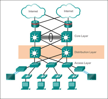
Cisco suggests a Three−Tier (Three Layer) hierarchical network model, that consists of three layers: the Core layer, the Distribution layer, and the Access layer. Cisco Three-Layer network model is the preferred approach to network design.

The above picture can further explained based on below picture.
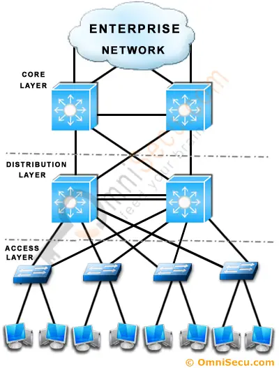
Core Layer
Core Layer consists of biggest, fastest, and most expensive routers with the highest model numbers and Core Layer is considered as the back bone of networks. Core Layer routers are used to merge geographically separated networks. The Core Layer routers move information on the network as fast as possible. The switches operating at core layer switches packets as fast as possible.
Distribution layer:
The Distribution Layer is located between the access and core layers. The purpose of this layer is to provide boundary definition by implementing access lists and other filters. Therefore the Distribution Layer defines policy for the network. Distribution Layer include high-end layer 3 switches. Distribution Layer ensures that packets are properly routed between subnets and VLANs in your enterprise.
Access layer
Access layer includes acces switches which are connected to the end devices (Computers, Printers, Servers etc). Access layer switches ensures that packets are delivered to the end devices.
Benefits of Cisco Three-Layer hierarchical model
The main benefits of Cisco Three-Layer hierarchical model is that it helps to design, deploy and maintain a scalable, trustworthy, cost effective hierarchical internetwork.
Better Performance: Cisco Three Layer Network Model allows in creating high performance networks
Better management & troubleshooting: Cisco Three Layer Network Model allows better network management and isolate causes of network trouble.
Better Filter/Policy creation and application: Cisco Three Layer Network Model allows better filter/policy creation application.
Better Scalability: Cisco Three Layer Network Model allows us to efficiently accomodate future growth.
Better Redundancy: Cisco Three Layer Network Model provides better redundancy. Multiple links across multiple devices provides better redundancy. If one switch is down, we have another alternate path to reach the destination.
another source : http://www.ciscopress.com/articles/article.asp?p=2202410&seqNum=4
Hierarchical Network Design Overview (1.1)
The Cisco hierarchical (three-layer) internetworking model is an industry wide adopted model for designing a reliable, scalable, and cost-efficient internetwork. In this section, you will learn about the access, distribution, and core layers and their role in the hierarchical network model.
Enterprise Network Campus Design (1.1.1)
An understanding of network scale and knowledge of good structured engineering principles is recommended when discussing network campus design.
Network Requirements (1.1.1.1)
When discussing network design, it is useful to categorize networks based on the number of devices serviced:
- Small network: Provides services for up to 200 devices.
- Medium-size network: Provides services for 200 to 1,000 devices.
- Large network: Provides services for 1,000+ devices.
Network designs vary depending on the size and requirements of the organizations. For example, the networking infrastructure needs of a small organization with fewer devices will be less complex than the infrastructure of a large organization with a significant number of devices and connections.
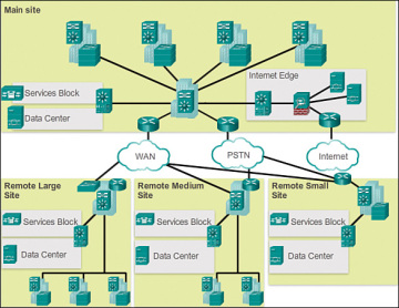
There are many variables to consider when designing a network. For instance, consider the example in Figure 1-1. The sample high-level topology diagram is for a large enterprise network that consists of a main campus site connecting small, medium, and large sites.
Network design is an expanding area and requires a great deal of knowledge and experience. The intent of this section is to introduce commonly accepted network design concepts.
NOTE
The Cisco Certified Design Associate (CCDA®) is an industry-recognized certification for network design engineers, technicians, and support engineers who demonstrate the skills required to design basic campus, data center, security, voice, and wireless networks.
Structured Engineering Principles (1.1.1.2)
Regardless of network size or requirements, a critical factor for the successful implementation of any network design is to follow good structured engineering principles. These principles include
- Hierarchy: A hierarchical network model is a useful high-level tool for designing a reliable network infrastructure. It breaks the complex problem of network design into smaller and more manageable areas.
- Modularity: By separating the various functions that exist on a network into modules, the network is easier to design. Cisco has identified several modules, including the enterprise campus, services block, data center, and Internet edge.
- Resiliency: The network must remain available for use under both normal and abnormal conditions. Normal conditions include normal or expected traffic flows and traffic patterns, as well as scheduled events such as maintenance windows. Abnormal conditions include hardware or software failures, extreme traffic loads, unusual traffic patterns, denial-of-service (DoS) events, whether intentional or unintentional, and other unplanned events.
- Flexibility: The ability to modify portions of the network, add new services, or increase capacity without going through a major forklift upgrade (i.e., replacing major hardware devices).
To meet these fundamental design goals, a network must be built on a hierarchical network architecture that allows for both flexibility and growth.
Hierarchical Network Design (1.1.2)
This topic discusses the three functional layers of the hierarchical network model: the access, distribution, and core layers.
Network Hierarchy (1.1.2.1)
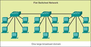
Early networks were deployed in a flat topology as shown in Figure 1-2.
Hubs and switches were added as more devices needed to be connected. A flat network design provided little opportunity to control broadcasts or to filter undesirable traffic. As more devices and applications were added to a flat network, response times degraded, making the network unusable.
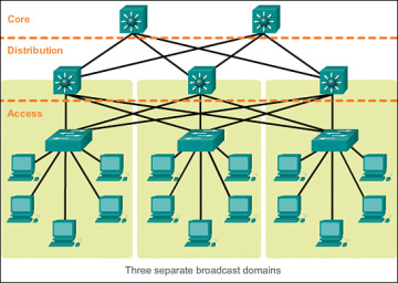
A better network design approach was needed. For this reason, organizations now use a hierarchical network design as shown in Figure 1-3.
A hierarchical network design involves dividing the network into discrete layers. Each layer, or tier, in the hierarchy provides specific functions that define its role within the overall network. This helps the network designer and architect to optimize and select the right network hardware, software, and features to perform specific roles for that network layer. Hierarchical models apply to both LAN and WAN design.
The benefit of dividing a flat network into smaller, more manageable blocks is that local traffic remains local. Only traffic that is destined for other networks is moved to a higher layer. For example, in Figure 1-3 the flat network has now been divided into three separate broadcast domains.
A typical enterprise hierarchical LAN campus network design includes the following three layers:
- Access layer: Provides workgroup/user access to the network
- Distribution layer: Provides policy-based connectivity and controls the boundary between the access and core layers
- Core layer: Provides fast transport between distribution switches within the enterprise campus
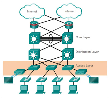
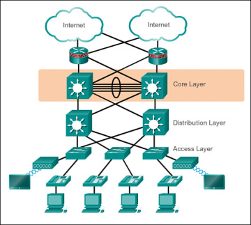
Another sample three-layer hierarchical network design is displayed in Figure 1-4. Notice that each building is using the same hierarchical network model that includes the access, distribution, and core layers.
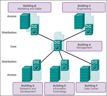 Figure 1-4 Multi Building Enterprise Network Design
NOTE
There are no absolute rules for the way a campus network is physically built. While it is true that many campus networks are constructed using three physical tiers of switches, this is not a strict requirement. In a smaller campus, the network might have two tiers of switches in which the core and distribution elements are combined in one physical switch. This is referred to as a collapsed core design.
The Access Layer (1.1.2.2)
In a LAN environment, the access layer highlighted grants end devices access to the network. In the WAN environment, it may provide teleworkers or remote sites access to the corporate network across WAN connections.
As shown in Figure 1-5, the access layer for a small business network generally incorporates Layer 2 switches and access points providing connectivity between workstations and servers.
The access layer serves a number of functions, including
- Layer 2 switching
- High availability
- Port security
- QoS classification and marking and trust boundaries
- Address Resolution Protocol (ARP) inspection
- Virtual access control lists (VACLs)
- Spanning tree
- Power over Ethernet (PoE) and auxiliary VLANs for VoIP
The Distribution Layer (1.1.2.3)
The distribution layer aggregates the data received from the access layer switches before it is transmitted to the core layer for routing to its final destination. In Figure 1-6, the distribution layer is the boundary between the Layer 2 domains and the Layer 3 routed network.
The distribution layer device is the focal point in the wiring closets. Either a router or a multilayer switch is used to segment workgroups and isolate network problems in a campus environment.
A distribution layer switch may provide upstream services for many access layer switches.
The distribution layer can provide
- Aggregation of LAN or WAN links.
- Policy-based security in the form of access control lists (ACLs) and filtering.
- Routing services between LANs and VLANs and between routing domains (e.g., EIGRP to OSPF).
- Redundancy and load balancing.
- A boundary for route aggregation and summarization configured on interfaces toward the core layer.
- Broadcast domain control, because routers or multilayer switches do not forward broadcasts. The device acts as the demarcation point between broadcast domains.
The Core Layer (1.1.2.4)
The core layer is also referred to as the network backbone. The core layer consists of high-speed network devices such as the Cisco Catalyst 6500 or 6800. These are designed to switch packets as fast as possible and interconnect multiple campus components, such as distribution modules, service modules, the data center, and the WAN edge.
As shown in Figure 1-7, the core layer is critical for interconnectivity between distribution layer devices (for example, interconnecting the distribution block to the WAN and Internet edge).
The core should be highly available and redundant. The core aggregates the traffic from all the distribution layer devices, so it must be capable of forwarding large amounts of data quickly.
Considerations at the core layer include
- Providing high-speed switching (i.e., fast transport)
- Providing reliability and fault tolerance
- Scaling by using faster, and not more, equipment
- Avoiding CPU-intensive packet manipulation caused by security, inspection, quality of service (QoS) classification, or other processes
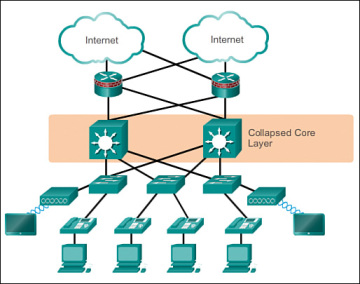
Two-Tier Collapsed Core Design (1.1.2.5)
The three-tier hierarchical design maximizes performance, network availability, and the ability to scale the network design.
However, many small enterprise networks do not grow significantly larger over time. Therefore, a two-tier hierarchical design where the core and distribution layers are collapsed into one layer is often more practical. A “collapsed core” is when the distribution layer and core layer functions are implemented by a single device. The primary motivation for the collapsed core design is reducing network cost, while maintaining most of the benefits of the three-tier hierarchical model.
The example in Figure 1-8 has collapsed the distribution layer and core layer functionality into multilayer switch devices.
The hierarchical network model provides a modular framework that allows flexibility in network design and facilitates ease of implementation and troubleshooting.
Activity 1.1.2.6: Identify Hierarchical Network Characteristics
Feb 11, 2016 | ccna, csico, exam, Learn and Teach, OSPF, Quiz, Routing Protocol, test
CCNP ROUTE Practice Exam Questions:
source: http://www.thebryantadvantage.com/CCNPExamBSCIPracticeExamMultiAreaOSPF3.htm
Multi-Area OSPF (Set #3)
Links to the other OSPF multiarea practice exams can be found at the end of the answers to this one.
As always with my practice exams, all multiple choice questions are “select all that apply”. Let’s get started!
Question 1:
The cost of an E2 route indicates what?
A. The cost of the path from the local router to the ASBR.
B. The cost of the path from the ASBR to the destination network.
C. The full cost of the path to the destination network from the local router.
D. The cost of the path from the ABR to the destination network.
Question 2:
What LSA type (numeric value) is generated by an ABR and describes inter-area links?
Question 3:
The cost of an E1 route indicates which of the following?
A. The cost of the path from the local router to the ASBR.
B. The cost of the path from the ASBR to the destination network.
C. The cost of the path from the local router to the destination network.
D. The cost of the path from the ASBR to the destination network.
Question 4:
By default, how does an OSPF routing table indicate routes that were injected into the OSPF domain via redistribution?
A. O EX
B. O *IA
C. O E2
D. O E1
E. O N2
Question 5:
Which of the following commands will show whether a router’s neighbors are or are not an ABR or ASBR?
A. show ip ospf database
B. show ip route ospf
C. show ip ospf neighbors
D. show ip ospf border-routers
Question 6:
You see a route marked “O IA” in your Cisco routing table. You know what the “O” stands for, or you wouldn’t be taking this exam. 🙂
However, what does the “IA” indicate regarding the destination network?
A. It’s in the same area as the local router.
B. It’s in another area.
C. It will be reached via a default route.
D. The route was learned via route redistribution.
Question 7:
What’s the number of the LSA type that is generated by every router for every area it belongs to, and is flooded to a single area?
Answers:
1. “B”. The default setting for a route learned by OSPF via redistribution is E2, and the metric of an E2 route is only the cost of the path from the ASBR to the destination network.
2. Type 3 LSAs are generated by ABRs and describe inter-area routes.
3. “C”. OSPF E1 routes reflect the entire cost of the path from the local router to the destination network.
4. “C”. As mentioned in the answer to Question 1. 🙂
5. “D”. It’s not one of the most common OSPF commands, but you can get some important information from the show ip ospf border-routers command.
6. “B”. The “IA” indicates a network that is in another OSPF area.
7. Type 1 LSAs are generated by every router for every area that it belongs to, and these LSAs are never flooded outside that particular area.
Thanks for taking this CCNP practice exam – here are the other OSPF multiarea exams on the site!
Feb 11, 2016 | Uncategorized
Administrative Distance for all routing protocol
Introduction
Most routing protocols have metric structures and algorithms that are not compatible with other protocols. In a network with multiple routing protocols, the exchange of route information and the capability to select the best path across the multiple protocols are critical.
Administrative distance is the feature that routers use in order to select the best path when there are two or more different routes to the same destination from two different routing protocols. Administrative distance defines the reliability of a routing protocol. Each routing protocol is prioritized in order of most to least reliable (believable) with the help of an administrative distance value.
Prerequisites
Requirements
Cisco recommends that you have knowledge of these topics:
Components Used
This document is not restricted to specific software and hardware versions.
Conventions
Refer to Cisco Technical Tips Conventions for more information on document conventions.
Select the Best Path
Administrative distance is the first criterion that a router uses to determine which routing protocol to use if two protocols provide route information for the same destination. Administrative distance is a measure of the trustworthiness of the source of the routing information. Administrative distance has only local significance, and is not advertised in routing updates.
Note: The smaller the administrative distance value, the more reliable the protocol. For example, if a router receives a route to a certain network from both Open Shortest Path First (OSPF) (default administrative distance – 110) and Interior Gateway Routing Protocol (IGRP) (default administrative distance – 100), the router chooses IGRP because IGRP is more reliable. This means the router adds the IGRP version of the route to the routing table.
If you lose the source of the IGRP-derived information (for example, due to a power shutdown), the software uses the OSPF-derived information until the IGRP-derived information reappears.
Default Distance Value Table
This table lists the administrative distance default values of the protocols that Cisco supports:
| Route Source |
Default Distance Values |
| Connected interface |
0 |
| Static route |
1 |
| Enhanced Interior Gateway Routing Protocol (EIGRP) summary route |
5 |
| External Border Gateway Protocol (BGP) |
20 |
| Internal EIGRP |
90 |
| IGRP |
100 |
| OSPF |
110 |
| Intermediate System-to-Intermediate System (IS-IS) |
115 |
| Routing Information Protocol (RIP) |
120 |
| Exterior Gateway Protocol (EGP) |
140 |
| On Demand Routing (ODR) |
160 |
| External EIGRP |
170 |
| Internal BGP |
200 |
| Unknown* |
255 |
* If the administrative distance is 255, the router does not believe the source of that route and does not install the route in the routing table.
When you use route redistribution, occasionally you need to modify the administrative distance of a protocol so that it takes precedence. For example, if you want the router to select RIP-learned routes (default value 120) rather than IGRP-learned routes (default value 100) to the same destination, you must increase the administrative distance for IGRP to 120+, or decrease the administrative distance of RIP to a value less than 100.
You can modify the administrative distance of a protocol through the distance command in the routing process subconfiguration mode. This command specifies that the administrative distance is assigned to the routes learned from a particular routing protocol. You need to use this procedure generally when you migrate the network from one routing protocol to another, and the latter has a higher administrative distance. However, a change in the administrative distance can lead to routing loops and black holes. So, use caution if you change the administrative distance.
Here is an example that shows two routers, R1 and R2, connected through Ethernet. The loopback interfaces of the routers are also advertised with RIP and IGRP on both the routers. You can observe that the IGRP routes are preferred over the RIP routes in the routing table because the administrative distance is 100.
R1#show ip route

Gateway of last resort is not set

172.16.0.0/24 is subnetted, 1 subnets
C 172.16.1.0 is directly connected, Ethernet0
I 10.0.0.0/8 [100/1600] via 172.16.1.200, 00:00:01, Ethernet0
C 192.168.1.0/24 is directly connected, Loopback0

R2#show ip route

Gateway of last resort is not set

172.16.0.0/24 is subnetted, 1 subnets
C 172.16.1.0 is directly connected, Ethernet0
C 10.0.0.0/8 is directly connected, Loopback0
I 192.168.1.0/24 [100/1600] via 172.16.1.100, 00:00:33,
In order to enable the router to prefer RIP routes to IGRP, configure the distance command on R1 like this:
R1(config)#router rip
R1(config-router)#distance 90
Now look at the routing table. The routing table shows that the router prefers the RIP routes. The router learns RIP routes with an administrative distance of 90, although the default is 120. Note that the new administrative distance value is relevant only to the routing process of a single router (in this case R1). R2 still has IGRP routes in the routing table.
R1#show ip route

Gateway of last resort is not set

172.16.0.0/24 is subnetted, 1 subnets
C 172.16.1.0 is directly connected, Ethernet0
R 10.0.0.0/8 [90/1] via 172.16.1.200, 00:00:16, Ethernet0
C 192.168.1.0/24 is directly connected, Loopback0

R2#show ip route

Gateway of last resort is not set

172.16.0.0/24 is subnetted, 1 subnets
C 172.16.1.0 is directly connected, Ethernet0
C 10.0.0.0/8 is directly connected, Loopback0
I 192.168.1.0/24 [100/1600] via 172.16.1.100, 00:00:33,
There are no general guidelines to assign administrative distances because each network has varied requirements. You must determine a reasonable matrix of administrative distances for the network as a whole.
Other Applications of Administrative Distance
One common reason to change the administrative distance of a route is when you use Static Routes to backup and existing IGP route. This is normally used to bring up a backup link when the primary fails.
For example, assume that you use the routing table from R1. However, in this case, there is also an ISDN line that you can use as a backup if the primary connection fails. Here is an example of a Floating Static for this route:
ip route 10.0.0.0 255.0.0.0 Dialer 1 250

!--- Note: The Administrative Distance is set to 250.
If the Ethernet interfaces fail, or if you manually bring down the Ethernet interfaces, the floating static route is installed into the routing table. All traffic destined for the 10.0.0.0/8 network is then routed out of the Dialer 1 interface and over the backup link. The routing table appears similar to this after the failure:
R1#show ip route
Gateway of last resort is not set
172.16.0.0/24 is subnetted, 1 subnets
C 172.16.1.0 is directly connected, Ethernet0
S 10.0.0.0/8 is directly connected, Dialer1
C 192.168.1.0/24 is directly connected, Loopback0
For more detailed information on the use of Floating Static routes, refer to these documents: